Graphical Representation of Discrete time Signals
Graphically, a discrete time signal can be represented using stem. This comaand shows the data in the form of samples (stems) starting from the baseline along x-axis and terminates each line in a circle or other marker.
The syntax is :
stem(a);
stem(t,a);
stem(t,a,'fill');
stem(t,a,'fill,'--')
stem(a) plots given data sequence a as stems along x-axis at equally spaced and automatically generated values.
stem(t,a) plots values of t versus the columns of a.
t and a must be the vectors or matrices of same size.
stem(t,x,'fill') will plot similar to above with ending circles filled.
stem(t,x,'fill','-') will plot similar to above with circles filled and dashed lines.
Example:
plot the signal x=sin(t) using stem command.
t=linspace(-pi,pi,15);
%fifteen equidistant instants between -pi to pi.
y=sin(t);
stem(t,y); % output is shown in Fig-1.
% for filled circles
t=linspace(-pi,pi,15);
y=sin(t);
stem(t,y,'fill'); % output is shown in Fig-2
% for filled circles and dashed
lines
t=linspace(-pi,pi,15);
y=sin(t);
stem(t,y,'fill', '--'); % output is shown in Fig-3
Basic discrete time signals.
1. Unit impulse signal
2. Unit step signal
3. unit ramp signal
4. Real valued exponential discrete time signal
5. Complex valued exponential discrete time signal
(No built in function is available in MATLAB for these basic functions)
1. Unit impulse signal 𝛿(n)
Example:
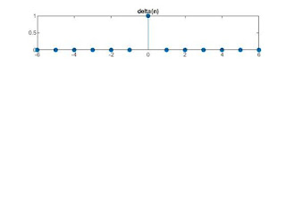
1) 𝛿(n) for -6<=n<=6
2) 𝛿(n+4) for -8<=n<=8
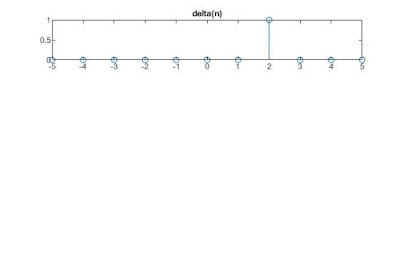
3) 𝛿(n-2) for -5<=n<=5
1) n=-6:6;
delta=1.*(n==0);
subplot(411);stem(n,delta,’fill’);
title(’delta(n)’);
2) n=-8:8; delta=1.*(n==-4);
subplot(411);stem(n,delta,’fill’);
title(’delta(n)’);
 3) n=-5:5; delta=1.*(n==2);
subplot(411);
stem(n,delta);
Graphically, a discrete time signal can be represented using stem. This comaand shows the data in the form of samples (stems) starting from the baseline along x-axis and terminates each line in a circle or other marker.
The syntax is :
stem(a);
stem(t,a);
stem(t,a,'fill');
stem(t,a,'fill,'--')
stem(a) plots given data sequence a as stems along x-axis at equally spaced and automatically generated values.
stem(t,a) plots values of t versus the columns of a.
t and a must be the vectors or matrices of same size.
stem(t,x,'fill') will plot similar to above with ending circles filled.
stem(t,x,'fill','-') will plot similar to above with circles filled and dashed lines.
 |
| Fig.-1 |
Example:
plot the signal x=sin(t) using stem command.
t=linspace(-pi,pi,15);
%fifteen equidistant instants between -pi to pi.
y=sin(t);
stem(t,y); % output is shown in Fig-1.
 |
| Fig.-2 |
% for filled circles
t=linspace(-pi,pi,15);
y=sin(t);
stem(t,y,'fill'); % output is shown in Fig-2
 |
| Fig.-3 |
% for filled circles and dashed
lines
t=linspace(-pi,pi,15);
y=sin(t);
stem(t,y,'fill', '--'); % output is shown in Fig-3
Basic discrete time signals.
1. Unit impulse signal
2. Unit step signal
3. unit ramp signal
4. Real valued exponential discrete time signal
5. Complex valued exponential discrete time signal
(No built in function is available in MATLAB for these basic functions)
1. Unit impulse signal 𝛿(n)
Example:
1) 𝛿(n) for -6<=n<=6
2) 𝛿(n+4) for -8<=n<=8
3) 𝛿(n-2) for -5<=n<=5
1) n=-6:6;
delta=1.*(n==0);
subplot(411);stem(n,delta,’fill’);
title(’delta(n)’);
2) n=-8:8; delta=1.*(n==-4);
subplot(411);stem(n,delta,’fill’);
title(’delta(n)’);
 3) n=-5:5; delta=1.*(n==2);
subplot(411);
stem(n,delta);
title(’delta(n)’);


Comments
Post a Comment